Numerical modeling of hurricane wind fields has long been used in severe wind impact studies, hurricane-induced storm surge and flooding predictions, and risk assessment studies. Storm surges are primarily induced by the surface wind stresses and secondarily by atmospheric pressure perturbations over shallow water in coastal areas. The accuracy of the storm surge predictions depends on how accurate are the atmospheric predictions that force the ocean and wave models. The use of full physics and high resolution mesoscale/regional atmospheric models might produce more accurate wind predictions but require extensive computing resources and simulation times to produce tropical cyclone (TC) forcing for storm surge forecasting and other hurricane related hazard studies. This is the exact reason that simple parametric TC models are widely used to generate the hurricane wind fields and to provide atmospheric forcing for storm surge and inundation forecasting. The advances made over the past several decades on improved hurricane track and intensity forecasts allow the parametric TC models to produce more accurate forecast in the region of the storm's path. The accuracy though of the parametric TC forecasts depends not only on the track and intensity, but also on the distribution of the wind field.

The development of PAHM follows the reasoning outlined above, and the philosophy of producing "accurate" wind fields quickly and effectively. PAHM contains various light-weight parametric tropical cyclone (TC) models that require minimal computational resources to produce the wind fields on the fly and fast. Such models use limited physics in producing "accurate" wind fields in the vicinity of the storm's path. The wind fields generated by these models are computed at the gradient level (Figure [7]). The gradient level is roughly \(300\,m \sim 3\,km\) above the surface of the earth (atop the atmospheric boundary layer, ABL), and is the level most representative of the air flow in the lower atmosphere immediately above the layer affected by surface friction. This level is free of local wind and topographic effects (such as sea breezes, downslope winds etc).

Figure 7: Schematic representation of the atmospheric boundary layer (ABL), its thickness variation over time and the definition of the gradient level. The conversion between the gradient level and the 10-m winds is denoted by the green arrow. This conversion can be achieved using the wind reduction factor \((w_{rf})\) or, an ABL model formulation.

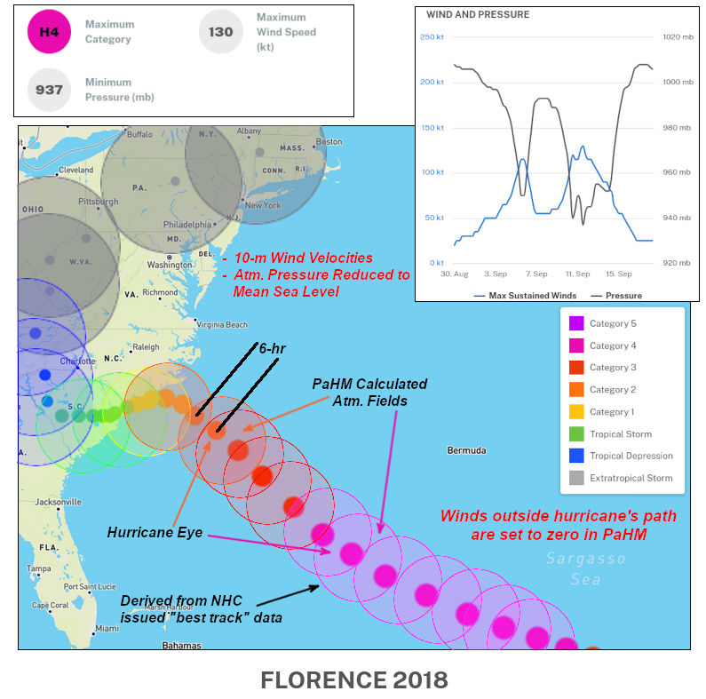
Figure 8: Calculation procedure of PaHM wind fields for Hurricane Florence (2018). Source of background images and track data: https://www.coast.noaa.gov/hurricanes/.

The 10-m wind may be estimated by decreasing the gradient level wind speed by approximately 10-20% over the ocean and up to 40% over land (wind reduction factor \(w_{rf}\) of 0.9-0.8 to 0.6 respectively). The use of a fixed and empiracally determined \(w_{rf}\) to convert the gradient winds to 10-m winds is a limitation of these models as \(w_{rf}\) is a function of location, time (ABL thickness is a function of time) and of course the characteristics of the particular TC.

Holland 1980

The traditional Holland Model (Holland 1980), thereafter HM80, is one of most widely used tropical cyclone (TC) analytical vortex models to generate meteorological forcings near the path of the storm. HM80 solves the reduced physics gradient wind equation \(\ref{eqn_holl80_grad_wind}\). Gradient winds are those theoretical winds that blow parallel to curved isobar lines or height-contour lines in the absence of turbulent drag (gradient level winds). The gradient level is roughly 1 km above the surface of the earth, and is the level most representative of the air flow in the lower atmosphere immediately above the layer affected by surface friction. This level is free of local wind and topographic effects (such as sea breezes, downslope winds etc) and it is commonly defined atop the atmospheric boundary layer (ABL).

For the gradient winds there is no balance between the Coriolis force and the Pressure gradient force (as this is the case for geostrophic winds), resulting in a non-zero net force \(F_{net}\) known as the Centripetal force. This \(F_{net}\) is what causes the wind to continually change direction as it goes around a circle (Stull 2017) as shown in Figures [9] and [10].

By describing this change in direction as causing an apparent force (Centrifugal), we can find the equation for the gradient wind. Equation \(\ref{eqn_holl80_grad_wind}\) defines the steady-state gradient wind and represents the balance of the Pressure Gradient Force \((F_{PG})\), Centrifugal \((F_{CN} = - F_{net})\) and Coriolis \((F_{CF})\) forces at the gradient level (Figures [9] and [10]):

\begin{equation} \underbrace{\vphantom{\frac{r}{\rho_{air}}\frac{\partial P(r)}{\partial r}} V^{2}_{g}(r)}_{F_{CN} \, \text{term}} + \underbrace{\vphantom{\frac{r}{\rho_{air}}\frac{\partial P(r)}{\partial r}} f r V_{g}(r)}_{F_{CF} \, \text{term}} - \underbrace{\frac{r}{\rho_{air}}\frac{\partial P(r)}{\partial r}}_{F_{PG} \, \text{term}} = 0 \label{eqn_holl80_grad_wind} \end{equation}

where: \(V_{g}(r)\) is the gradient level wind speed at radius \(r\), \(P(r)\) is the pressure at radius \(r\), \(r\) is the radial distance, \(f = 2 \Omega \sin\phi\) is the Coriolis parameter, \(\Omega = 7.27221\cdot 10^{-5} s^{-1}\) is the rotational speed of the earth, \(\phi\) is the latitude in radians and \(\rho_{air}\) is the air density (assumed constant: \(1.15 \, kg / m^3\)). The quadratic equation \(\ref{eqn_holl80_grad_wind}\) has two roots:

\begin{align} \label{eqn_holl80_grad_wind_rootsa} &V_{g}(r) = \sqrt{ \frac{r}{\rho_{air}}\frac{\partial P(r)}{\partial r} + \big(\frac{r f}{2}\big)^2} - \frac{r f}{2} \\[10pt] \label{eqn_holl80_grad_wind_rootsb} &V_{g}(r) = - \sqrt{ \frac{r}{\rho_{air}}\frac{\partial P(r)}{\partial r} + \big(\frac{r f}{2}\big)^2} - \frac{r f}{2} \end{align}

where equation \(\ref{eqn_holl80_grad_wind_rootsa}\) is the solution for \(V_{g}(r)\) for flow around a cyclone that is, around a low pressure (Figure [9]) while, equation \(\ref{eqn_holl80_grad_wind_rootsb}\) represents the solution for \(V_{g}(r)\) for flow around an anticyclone that is, around a high pressure (Figure [10]).

Figure 9: Forces that cause the gradient wind to be faster than geostrophic for an air parcel circling around a low-pressure center (a cyclone in N. Hemisphere). The centrifugal force pulls the air parcel inward to force the wind direction to change as needed for the wind to turn along a circular path. Source: Practical Meteorology: An Algebra-based Survey of Atmospheric Science. Roland Stull, The University of British Columbia, Vancouver, Canada.

Figure 10: Forces that cause the gradient wind to be faster than geostrophic for an air parcel circling around a high-pressure center (an anticyclone in the N. Hemisphere). The centrifugal force pulls the air parcel inward to force the wind direction to change as needed for the wind to turn along a circular path. Source: Practical Meteorology: An Algebra-based Survey of Atmospheric Science. Roland Stull, The University of British Columbia, Vancouver, Canada.

To derive the analytical expression for \(V_{g}(r)\), HM80 assumed a surface pressure profile that is approximated by the following hyperbolic equation:

\begin{equation} P(r) = P_{c} + (P_{n} - P_{c}) e^{-A/r^B} \label{eqn_holl80_hyp_pres_prof} \end{equation}

where: \(A, \, B\) are scaling parameters, \(P(r)\) is the pressure at radius \(r\), \(P_{n}\) is the ambient pressure (assumed constant: \(1013.25 \, mbar\)) and \(P_{c}\) is the central pressure. Substituting the expression for \(P(r)\) into equation \(\ref{eqn_holl80_grad_wind_rootsa}\) and, the following expression for the wind speed at the gradient level is obtained:

\begin{equation} V_{g}(r) = \sqrt{ A B (P_{n} - P_{c}) e^{-A/r^B} / \rho_{air} r^{B} + \big(\frac{r f}{2}\big)^2} - \frac{r f}{2} \label{eqn_holl80_vg} \end{equation}

To determine the scaling parameters \(A\) and \(B\), it is assumed that at the region of the radius of maximum winds (RMW) that is, at the region of the sustained maximum wind speeds \((r = R_{max} = \text{RMW})\), the wind speed \(V_{g}\) satisfies the first of equations \(\ref{eqn_holl80_asump}\). It is also assumed that the Rossby number \(R_{o}\) is very large (the third of equations \(\ref{eqn_holl80_asump}\)), so that the Coriolis forces can be neglected and therefore the air is in cyclostrophic balance (Holland 1980) as described by equation \(\ref{eqn_holl80_vg_cycl}\) for the cyclostrophic wind speed \(V_{c}(r)\).

\begin{equation} V_{g} = V_{max} \,;\quad \frac{dV_{g}}{dr} = 0 \,;\quad R_{o} = \frac{V_{max}}{f R_{max}} \gg 1 \label{eqn_holl80_asump} \end{equation}

\begin{equation} V_{c}(r) = V_{g}(r)\Big|_{r \rightarrow R_{max}} = \sqrt{ A B (P_{n} - P_{c}) e^{-A/r^B} / \rho_{air} r^{B}} \label{eqn_holl80_vg_cycl} \end{equation}

Applying the second of the conditions in equations \(\ref{eqn_holl80_asump}\) on equation \(\ref{eqn_holl80_vg_cycl}\), we find that the radius of maximum winds is independent of the relative values of the ambient and the central pressure and it is defined only by the scaling parameters \(A\) and \(B\) as: \(R_{max} = A^{1/B}\), or \(A = R_{max}^{B}\). Substituting the expression for \(A\) into equation \(\ref{eqn_holl80_vg_cycl}\) and setting \(V_{c}(R_{max}) = V_{max}\), the expression for the scaling parameter \(B\) (widely known as the Holland \(B\) parameter) is readily determined:

\begin{equation} A = R_{max}^{B} \,;\quad B = \frac{\rho_{air} e V_{max}^{2}}{P_{n} - P_{c}} \label{eqn_holl80_scale} \end{equation}

Physically, the Holland parameter \(B\) defines the shape of the pressure profile (equation \(\ref{eqn_holl80_hyp_pres_prof}\)) while, the parameter \(A\) determines its location relative to the origin (Holland 1980). HM80 states that plausible ranges of B would be between 1 and 2.5 to to limit the shape and size of the vortex. Based on equations \(\ref{eqn_holl80_hyp_pres_prof}\), \(\ref{eqn_holl80_vg}\) and \(\ref{eqn_holl80_scale}\), and re-organizing the pressure and the gradient wind speed equations, the final equations of the HM80 parametric TC model that PAHM solves are summarized as follows:

\begin{align} & B = \frac{\rho_{air} e V_{max}^{2}}{P_{n} - P_{c}} \label{eqn_holl80_b} \\[10pt] & P(r) = P_{c} + (P_{n} - P_{c}) \cdot e^{-(R_{max} / r)^{B}} \label{eqn_holl80_pres} \\[10pt] & V_{g}(r) = \sqrt{ V_{max}^{2} \cdot \big(\frac{R_{max}}{r}\big)^{B} \cdot e^{1 - (R_{max} / r)^{B}} + \big(\frac{r f}{2}\big)^2} - \frac{r f}{2} \label{eqn_holl80_vg1} \end{align}

As reasoned in Gao 2018, a large \(R_{o}\) \((\,\orderof{10^3}\,)\) describes a system in cyclostrophic balance dominated by inertial and centrifugal forces with negligible Coriolis force (e.g., a tornado or the inner core of an intense hurricane), while a small value \(R_{o}\) \((10^{-2} \sim 10^{2})\) describes a system in geostrophic balance strongly influenced by the Coriolis force (e.g., the outer region of a TC). Therefore, the cyclostrophic balance assumption made in HM80 is only valid for describing an intense but narrow TC with a large \(R_{o}\), and not suitable for weak but broad tropical cyclones with small \(R_{o}\) values. Although this is a limitation of the HM80 model, equations \(\ref{eqn_holl80_b}\) through \(\ref{eqn_holl80_vg1}\), are widely used in hurricane risk studies and storm surge studies due to their simplicitly and their capability to generate the atmospheric fields quickly and efficiently.

Generalized Asymmetric Vortex Holland model (GAHM)

The Generalized Asymmetric Vortex Holland model (Gao et al. 2015 and Gao 2018) extends HM80 by eliminating the cyclostrophic assumption at the the region of RMW (the third of equations \(\ref{eqn_holl80_asump}\)) to allow the generation of representative wind fields for a wider range of TCs. GAHM also introduces a composite wind methodology to fully use all multiple storm isotachs in TC forecast or best track data files to account for asymmetric tropical cyclones such as a land-falling hurricane.

GAHM model solves the gradient wind equation for \(V_{g}\) (equation \(\ref{eqn_holl80_grad_wind_rootsa}\)) by eliminating the influence of the Rossby number \((R_{o})\)) on the gradient wind solution assuming that:

\begin{equation} V_{g} = V_{max} \,;\qquad \frac{dV_{g}}{dr} = 0 \label{eqn_gahm_asump} \end{equation}

The pressure profile used is the same as in HM80 (equation \(\ref{eqn_holl80_hyp_pres_prof}\)) where the scaling parameter \(A\) is slightly re-defined by introducing a new scaling factor \((\phi)\) : \(\phi = A / R_{max}^{B}\), or \(A = \phi R_{max}^{B}\). Substituting the expression for \(A\) into equation \(\ref{eqn_holl80_vg}\) and using the second of equations \(\ref{eqn_gahm_asump}\), an adjusted Holland B parameter \((B_{g})\), is derived as:

\begin{equation} B_{g} = \frac{(V_{max}^{2} + f V_{max} R_{max}) \rho_{air} e^{\phi}}{\phi(P_{n} - P_{c})} = B \frac{(1 + 1 / R_{o}) e^{\phi - 1}}{\phi} \,;\qquad B = \frac{\rho_{air} e V_{max}^{2}}{P_{n} - P_{c}} \label{eqn_gahm_bg} \end{equation}

Substituting the expressions for \(A\) and \(B \, (\text{replaced by} \, B_{g})\) into equation \(\ref{eqn_holl80_vg}\) and using the first of equations \(\ref{eqn_gahm_asump}\), the final expression for the scaling parameter \(\phi\) is derived:

\begin{equation} \phi = \frac{1 + f V_{max} R_{max}}{B_{g}(V_{max}^{2} + f V_{max} R_{max})} = 1 + \frac{1 / R_{o}}{B_{g} (1 + 1/R_{o})} \label{eqn_gahm_phi} \end{equation}

Based on equations \(\ref{eqn_holl80_hyp_pres_prof}\), \(\ref{eqn_holl80_vg}\), \(\ref{eqn_gahm_bg}\), and \(\ref{eqn_gahm_phi}\) and re-organizing the pressure and the gradient wind speed equations, the final equations of the GAHM parametric TC model that PAHM solves are summarized as follows:

\begin{align} & B_{g} = B \big(1 + \frac{1}{R_{o}} \big)^{e^{-\phi} / \phi} \,;\quad \phi = 1 + \frac{1/R_{o}}{B_{g} (1 + 1/R_{o})} \,;\quad B = \frac{\rho_{air} e V_{max}^{2}}{P_{n} - P_{c}} \,;\quad \text{and} \quad R_{o} = \frac{V_{max}}{f R_{max}} \label{eqn_gahm_bg_phi} \\[10pt] & P(r) = P_{c} + (P_{n} - P_{c}) \cdot e^{-\phi (R_{max} / r)^{B_{g}}} \label{eqn_gahm_pres} \\[10pt] & V_{g}(r) = \sqrt{ V_{max}^{2} \cdot \big(\frac{R_{max}}{r}\big)^{B_{g}} \cdot (1 + 1/R_{o}) \cdot e^{\phi (1 - (R_{max} / r)^{B_{g}})} + \big(\frac{r f}{2}\big)^2} - \frac{r f}{2} \label{eqn_gahm_vg} \end{align}

Given the values for \(V_{max}\), \(R_{max}\), \(P_{n}\) and \(P_{c}\), the iterative solution of the first two of equations \(\ref{eqn_gahm_bg_phi}\) produces the final values of \(B_{g}\) and \(\phi\).

Table of Contents

Holland 1980

Generalized Asymmetric Vortex Holland model (GAHM)